About Linear Regression

tags: #ML/supervised/regression

What is linear regression?

Linear Regression ~ Ordinary Least Squares

Linear regression is also known as Ordinary Least Squares Multiple Linear Regression

"Linear" - bc the underlying relationship is assumed to be linear (this is also one of the assumptions for using linear regression), and the equation to model the relationship is based on the linear equation of: $y = m x + b$
"Least squares" - technique used to find the line of best fit
"Ordinary" - type of least squares method
"Multiple" - bc the regression can include more than 1 independent variable

The linear regression model is a statistical (and ML) model that can be applied to:

Any type of independent variable
A quantitative dependent variable
Can have more than 1 independent variable

Note: with regression models, you are predicting a real-valued number.

Assumptions Check: Linearity

We can check for the presence of linearity using a scatterplot:

If the data in the scatterplot approximates a straight line $\to$ indicates a linear relationship
When a linear relationship exists, Y can be predicted for any given value of X.
In a perfect linear relationship, all data values fall along a straight line exactly
However, most real-world data do not exhibit a perfect linear relationship $\to$ instead we can approximate a 'line of best fit' that minimizes prediction errors using the OLS method.
This line can be described mathematically based on the linear equation where $y = m x + b$

Understanding the "Line of Best Fit"

The goal of a regression model is to find a line of best fit that would minimize the difference between the predicted output ( $y$ ) and the real-valued $t$ for all data points to the regression line.

The equation of the line of best fit can be represented as:

y = m x + b

or...

y = b x + b_{0}

Interpreting the Equation

y - predicted value of the dependent variable

x - is the value of the independent variable

b0 - is the y-intercept (constant)

For quantitative variables: this represents the mean value of the response (y) variable when all of the predictor variables in the model are equal to zero.
For categorical variables: this represents the response of the dependent variable when all categorical variables are at reference level
may or may not have meaningful interpretation for the model depending on the context

b - is the slope of the line (regression coefficient)

most important value
represents the relationship between the IDV to the DV
is the measure of the change in Y for each unit change in X
i.e., for each unit increase in X, Y increases by the value of b
e.g., for y = 5 +2x - this means that for every unit increase in x, there is 2 unit increase in Y.

Approximating the Line of Best Fit: OLS

We can approximate the line of best fit using the ordinary least squares method:

Definition: Best fitting line

In the context of OLS, the best fitting line is the line where the residual sum of squares is at a minimum. This is our "loss function" for linear regression.

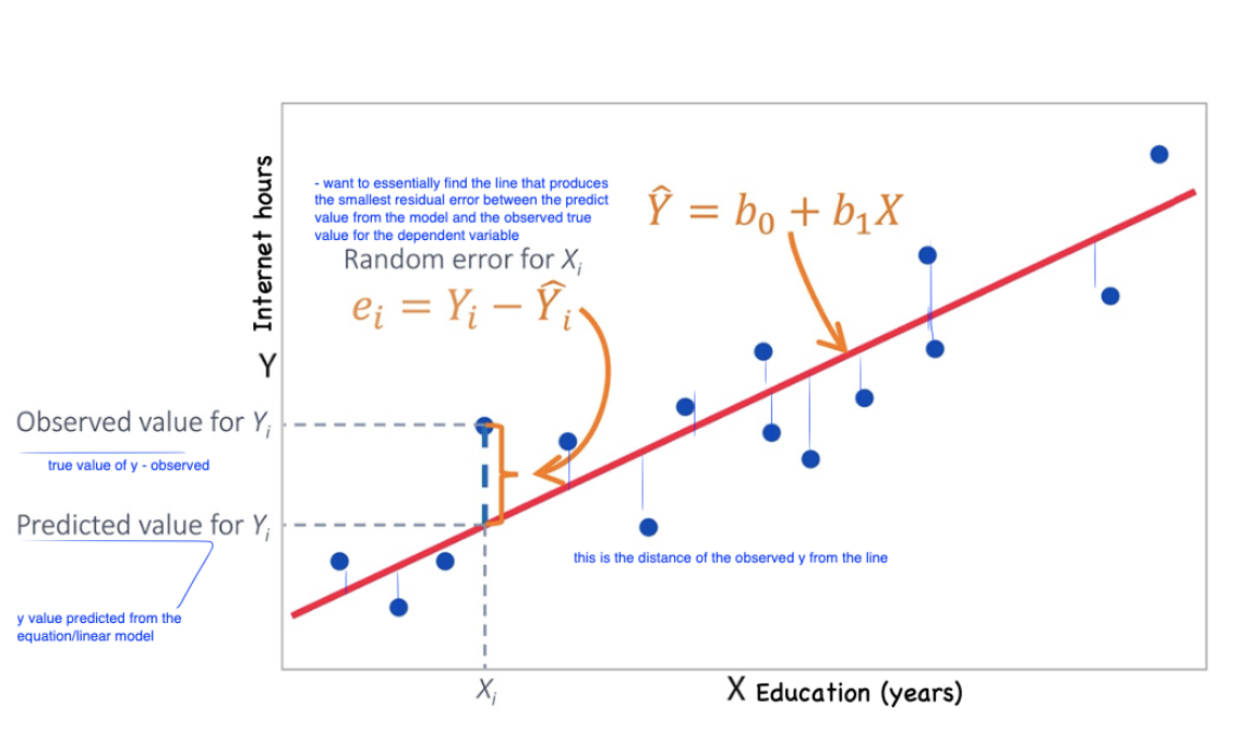
Therefore, a $S S_{r e s i d u a l s}$ of 0 is one that will produce the "best fitting line".

The least-sqaures method is the technique used to find the line of best fit by minimizing the sum of the squared residuals of each data point from the regression line, such that:

S S_{r e s i d u a l s} = \sum_{i = 1}^{n} (y_{i} - \hat{y_{i}})^{2}

The residual (AKA prediction error) is the difference between the observed Y and the predicted Y:

e = y - \hat{y}

Goal of linear regression is to find a line that minimizes the residual error each observation by adjusting the parameters of the linear equation in $y = a + b x$ that makes the sum of the squared residuals as small as possible:

Optimization Algorithm: Gradient Descent

This is achieved through an optimization algorithm called "gradient descent" used to find the best set of parameters (w, b), that minimizes the loss function by finding the global minima of the performance surface of the function.

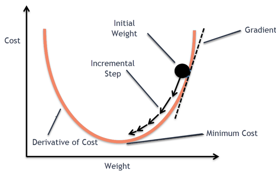
Screen Shot 2023-04-27 at 9.51.33 PM.png500

The lowest point on the performance surface correspond to the optimal set of parameters where the loss function is minimized and the accuracy is the highest.

Caveat! Works well when the function is convex, otherwise, the algorithm can get stuck at sub-optimal solutions ("saddle points" or "local minimas"). Not the case for linear regression as the loss function is convex, therefore, it has only one minimum point that is the global minima.

The line that produces the smallest sum of squares is the best fitting line

Illustration:

Screen Shot 2023-04-24 at 6.31.20 PM.png

Dummy Variables

See also: Dummy Encoding

For nominal variables that convey only classification information - we can create dummy variables for each class of a categorical variable; this allows for multiple comparisons to be made for each subgroup in a single regression model.

Each dummy variable is coded as 0 or 1 depending on whether that individual is in that category.

A regression model can have many dummy variables and be used as independent variables.

When dummy variables are used as dependent variables, we have binary or multi-class classification.

Additional Resources

INF2179 ML - Linear Regression Lecture